Technical Articles

The process simulation SIGMASOFT^® Virtual Molding is already a well-established tool in the development phase of elastomer products. It is used to prevent problems in the production and to shorten the time to market in industrial applications. Already very early in the development phase runner systems can be balanced or mold temperatures optimized. In spite of ongoing development and increasing complexity of the models it happens that the simulation results do not match the measurements at the machine.

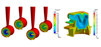
This does not only concern the simulated pressure, but also further results as the filling behavior and many temperature related results because of their correlation with pressure changes. Thus it becomes not only more difficult to decide whether the part fills as predicted, but also results as curing degree, mechanical properties of the part, material degradation or warpage of the part may become less reliable (Picture 1).

If the phenomena observed at the machine during serial production are not the same as the predicted values, major problems can occur. Lost money, time delay and frustrated customers are some of the consequences. The question now is why something like this happens and even more important how one can avoid problems like this.

One of the key values during mold design is the pressure needed to fill the cavity. The maximum pressure is one of the limiting factors for the machine selection. It is also an indicator for the energy that heats up the elastomer during filling and is therefore critical for the curing time prediction.

Pressure can be measured at various positions in the system. Hydraulic pressure, pressure sensors in the piston or the mold are most common references for the pressure. Usually only one reference is used. If the system offers more than one measured pressure, the values are often already contradictory.

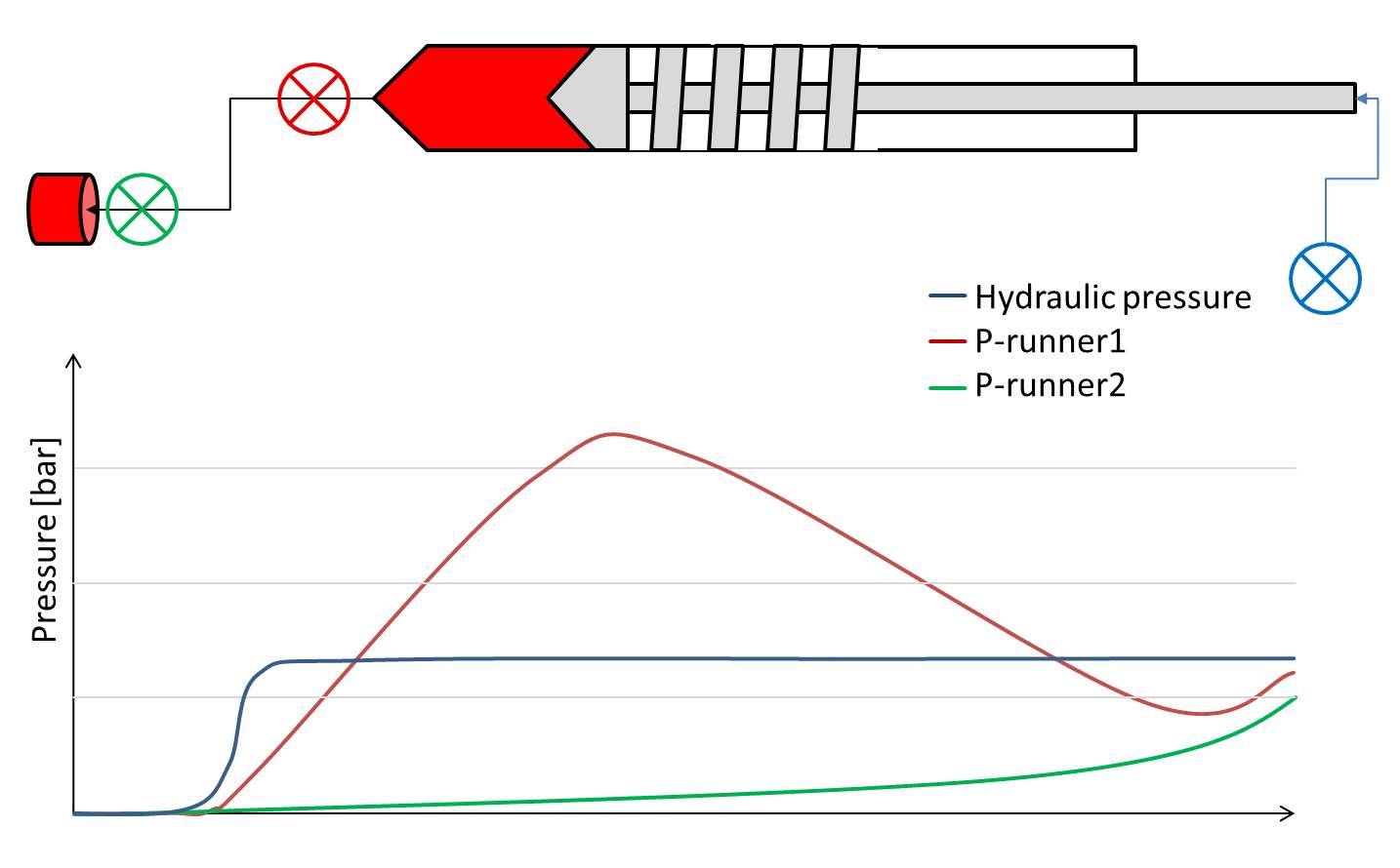
Picture 2 shows the measured pressure at two different points in the gating system of an elastomer mold. Even though the hydraulic pressure is constant, the pressure close to the machine (P-runner1) decreases at a certain point. On the first view it looks unphysical. What happened in this case is that the hydraulic pressure also sees what happens in the piston. If the melt cushion becomes too small, the flow behavior in this area can dramatically increase the hydraulic pressure.

In the simulation the pressure can be predicted at various positions as well. In addition the simulation is usually based on different models and ideal boundary conditions. Due to the selected model and the assumptions for the process simulation results can vary. These variations are based on the complex interaction between material measuring errors, modeling and assumptions. Therefore the results are often hard to judge.

One of the critical values for the prediction of the pressure is the viscosity depending on shear rate and temperature. Unfortunately there is no way to directly measure the viscosity. Depending on the system that is used, pressure or momentum are measured at specific conditions of flow. Based on these values and several corrections, the viscosity can be calculated. Since the setup of these systems is very sensitive the results can vary in a wide range. Especially for elastomer mixtures these scatter of measured viscosity can be more than 100%. 

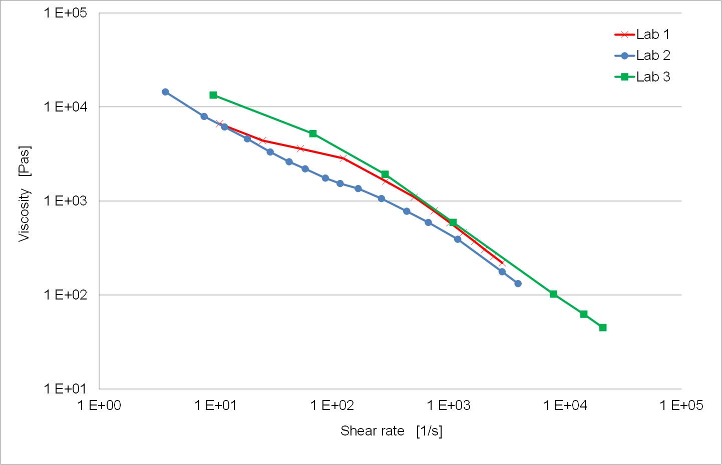
Picture 3 shows the result of three different measurements for one mixture (one batch), measured at three different laboratories. The diagram is plotted in logarithm scale. The viscosity measured at laboratory three is 5 times higher than the viscosity measured at laboratory 2. If these viscosities are used in a simulation, the predicted pressure will be completely different for the three measurements.

One reason for these differences is the sensitivity of high pressure viscometers. Depending on how the elastomer is placed in the machine and depending on the setup of the system the measured results can vary a lot.

Other effects are the various corrections which can be used to calculate the true viscosity (Weissenberg-Rabinowitsch, Mooney, Bagley). These corrections usually need a more complex setup or different experiments. Since every experiment has to be paid, not all of the corrections are done in every characterization.

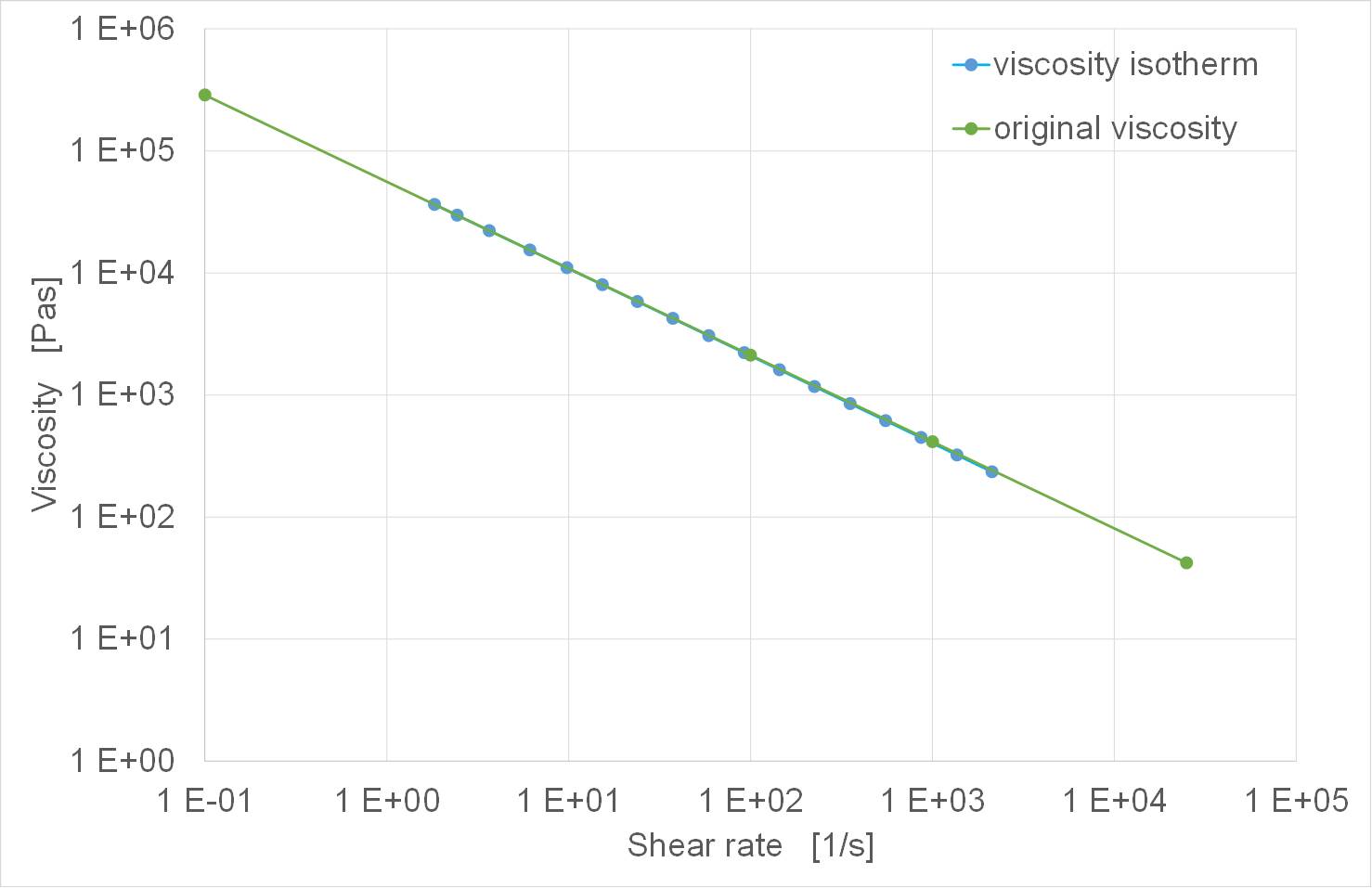
In addition to the already complex problem of known corrections, there is no correction taking into account the temperature increase during the measurement. The material is pushed through a capillary with a high pressure. The higher pressure and velocity are the higher the shear heating will be. Depending on the sensitivity of the viscosity for temperature changes the real viscosity will be a lot higher than the measured viscosity. Picture 4 shows a virtual experiment. In this experiment a material with a certain viscosity (original viscosity) is used to simulate a high pressure capillary viscometer. The simulated pressure is used to calculate the viscosity as it is done in the real experiment. The second curve (viscosity isotherm) shows the calculated viscosity based on this experiment. The material used to generate the viscosity was modified in the simulation in a way that the temperature couldn’t increase. One can see that both curves match pretty good. This proof of concept shows that the simulation of the capillary works very accurate and gives the correct pressure prediction.

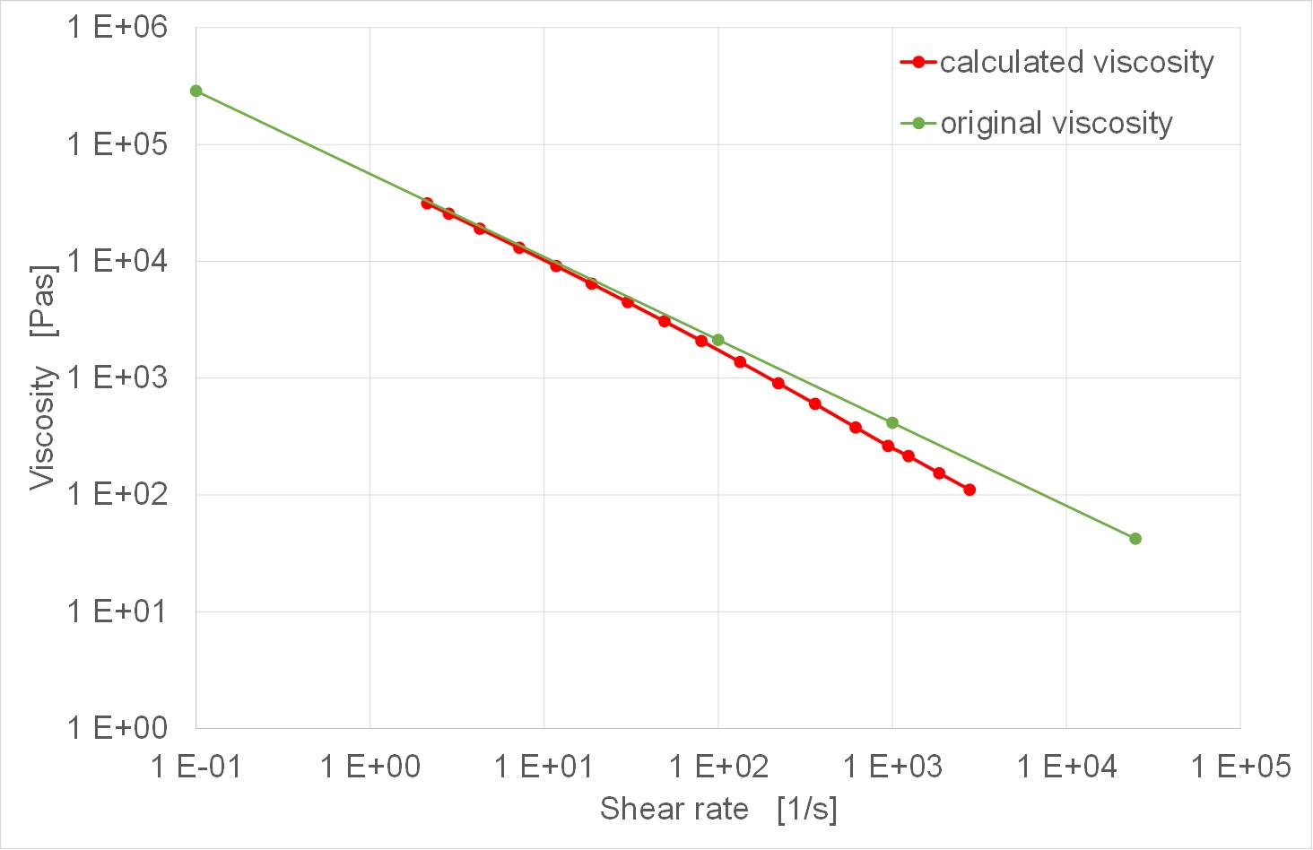
A second simulation was performed. In this simulation the material was allowed to change the temperature due to shear heating. Again the viscosity was calculated. Picture 5 shows the original viscosity (green curve) and the calculated viscosity (red curve) for this material. In the region of low shear rates the two curves match very well. In these areas the shear heating is rather low so the material does not heat up too much. In the region of higher shear rates the distance between the two curves become bigger. At the shear rate of 1000/s the difference between the two curves is approximately a factor of two. This simple experiment shows the dramatic influence of the temperature increase during the viscosity measurement. To predict the pressure loss in an elastomer mold it is necessary to also correct this behavior.

One way to get the real viscosities is a simulation. SIGMASOFT^® Virtual Molding can be used to find the real viscosity taking the temperature increase into account.

This short introduction in measuring and simulating pressure shows that that there are various questions that have to be answered in detail before the simulation result will match the measured pressure. It is not always necessary to answer all of these questions but it is important to be aware of the influence of certain effects. This will make sure that critical values can be avoided in the production.